You are not the average player
(May 2022 edit): This forum post1 (and the series of posts it links to) is possibly more relevant than this whole discussion.
I recently decided to learn more about economy. Having a physics background, I was happy to discover that physicists are known for criticizing what they think are the economists' vision2. I was happy partly because I like being the party’s arrogant physicist, and partly because I think reading outsiders' criticism is a useful way of learning more about a research area.
Ole Peters is one of the regular critiques of economy3. While I am not sure Peters' vision is particularly useful in itself, I was happy to reflect on a simple example he provides4. In this article, I want to exploit the explanatory power of the model to go through some basic decision theory and finance concepts. Before moving on, I note that this model is very similar to the St. Petersburg paradox5, and has already been nicely discussed elsewhere6.
Peters' gamble
You start with a wealth of 100€. You can play the following game 10 times in a row: A coin is tossed. If it lands head, you win 50% of your current bankroll (ending up with 150€ after the first round). If it lands tail, you lose 40% of you current bankroll (ending up with 60€ after the first round).
Would you accept the deal and play the game 10 times, or rather keep your initial fortune?
The paradox
The gamble proposed above presents us with an apparent paradox. Say we start with $X_0$ dollars (above, $X_0 = 100€$). After playing a round of the game, we end up on average with: $$ X_1 = \frac{1}{2} W X_0 + \frac{1}{2} L X_0 $$ where $W = 1.5$ is the factor by which our wealth increases when we win, and $L = 0.6$ is the factor by which our wealth decreases when we lose. Plugging in the numbers, we see that $X_1 = 1.05 \times X_0$. In other words, our wealth will increase on average by 5% after a round. This applies to every round, so after 10 rounds our wealth should have increased by $(1.05)^{10}$: 63%. Not so bad, is it?
However, if you simulate a game, you will most likely find yourself having lost money after 10 rounds. What is happening here?
You are not the average player
So far we only looked at the average outcome, but you are not the average player. You are just one player, who, as you played the game, has walked along only one of the possible event paths. So, what we would really like to know is What is, on average, the outcome obtained by following a random path (chosen uniformly across the set of all paths)?. I will call this the typical outcome. How come the average outcome and the typical outcome can be different? How come the average player fares well, while the typical player looses money by accepting the gamble?
Typical paths
To answer, let us look at what a path typically is like.
What I call a path is the succesion of “win” and “loss” events a player encounters as he repetitively goes through rounds of the game.
For example, a path in a game of 10 rounds might look like: WWLWWLWLLL.
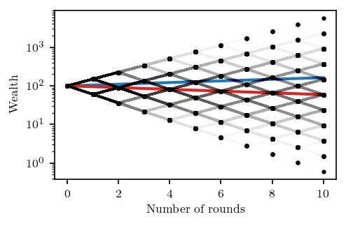
The figure above depicts the set of all possible paths. More precisely, each point represents a possible outcome of the game after playing the corresponding number of rounds. Points in consecutive rounds are connected by a segment if there a win/loss event connecting them. The opacity of a segment is proportional to the number of paths that contain the corresponding win/loss event.
As the figure illustrates, in the large number of rounds limit, almost all paths have the same number of W and L events.
I will call such paths balanced.
In the case were we play 10 rounds, balanced paths already make up 26% of the total.
On the figure, the closer a path is to being balanced, the closer it is to the red line.
Another important observation is that the outcome does not depend on the order of the letters along a path. In particular, picking any balanced path always leads to the same outcome. Since this class dominates the set of possibilities, this outcome is the typical outcome we were looking for! After 10 rounds, the typical outcome will be $(WL)^{5} \times X_0 = 59€$. Far from seeing our wealth increased by 63% like it does on average, we typically see it reduced by 41%! On the figure, the red line shows the typical outcome, while the blue line shows the average one.
If you are a casino manager, I would advise you not to set this game up. Not only will most of the players walk out of the casino having lost 41% of their entry ticket, but the casino itself will consistently lose money, due to the rare lucky players who make the average outcome of the game positive.
Cheating the game: financial market strategies
Another surprise to me was to find out that it is possible for players to win the game, only by slightly altering the rules. There are at least two ways. The first is obvious, the second less so.
Creating a portfolio
Don’t you find it unjust that a few lucky players walk out of the casino so outtrageously rich that they push the average outcome to 63% of the initial bet? Let us agree to split our outcomes equally: then we all win by 63%. In financial terms, this would be called a diversification strategy. Remark that it only works if the number of players more than matches the number of rounds. 10 players would end up all poor after 1000 rounds!
Saving money
What if I told you you could gain more by betting less? I guess it makes sense from a risk averse perspective, but I still find fascinating that it works. The strategy stems from the observation that the typical paths make us lose because walking them we encounter many “win/loss” couples, and $WL < 1$. However, by re-injecting only a fraction $\lambda$ of our bankroll $G_0$, we can hack the value of $W$ and $L$. Indeed, after winning, our bankroll becomes $$ G_1 = W \lambda G_0 + (1-\lambda) G_0 $$ By investing only a fraction $\lambda$, we’ve effectively replaced $W$ by $W' = W \lambda + 1 - \lambda$, and similarly in the “loss” case. Can the product $W’L'$ be larger than 1? Yes! Let’s be ambitious and maximise it. We do not simply want to win, we want to win as much as possible. This is achieved for $$ \lambda_\text{max} = \frac{1}{2} \left( \frac{1}{1-L} - \frac{1}{W - 1} \right) $$ We have recovered in a simple case the Kelly criterion7, a well-known asset management tool.
Putting it all together: utility functions
Can we explain all of the above in a single line? Yes! The average change in log-utility after a single round of the game is $$ \Delta U = \frac{1}{2} \log W + \frac{1}{2} \log L $$ We should accept the gamble only if it increases our utility on average. With the values of $W$ and $L$ given, it turns out that $\Delta U < 0$ (this is just equivalent to saying $WL < 1$). Since the total utility of the game is the sum of $\Delta U$ over the rounds, it is negative as well: A log-utility player will refuse the gamble.
Enters Ole Peters
The apparent paradox nicely illustrates the fact that it is generally a bad idea to just look at the average of a distribution. But Ole Peters sees more to it. He raises at least two points4:
- Utility function is just an obfuscated way of saying that players should “maximise the average growth rate”
- This game illustrates that some real world situations are “non-ergodic”, and should be treated as such (Peters goes on to argue that this point is lost on economists).
I will not comment more on those points. The interested reader can head to8 for a discussion about ergodicity, and9 for one about utility functions and growth rates.
Conclusion and further directions
I am amazed by the explanatory power of this extremely simple toy model. It is enough to generate wealth inequality, and naturally explains how risk aversion and asset diversification strategies arise. Perhaps unsurprinsingly, an immediate generalisation of the game, the geometric Brownian motion, has been used to model financial markets10.
I can imagine at least three ingredients this models lacks.
- There is no memory effect: For example, even players who at a given point in time fare extremely well are ultimately doomed to lose. Real life is seemingly different: accumulated wealth seems relatively stable,
- There is no noise or uncertainty built in the model,
- There are no interactions between the players.
What can we say about individual or collective decision making once these elements are added to the picture?